Goalkeeper Expected Saves

Expected Goals (xG) has been all the craze within soccer analytics the last few years, but what if we changed perspectives. For every shot on target, I wanted to know the probability of that shot being saved, hence expected saves. I want to give a big shoutout to Alfian Hakim and his article, How to Build Your Own Expected Goals (xG) Model. Much of my code structure with the use of StatsBomb data and the visualizations are based on his code that he provided.
For this analysis, I used StatsBomb’s data for all 64 matches played in the 2022 FIFA Men’s World Cup. First let’s look at some visuals related to shots on target.

Every shot on target, based on field position, and its result
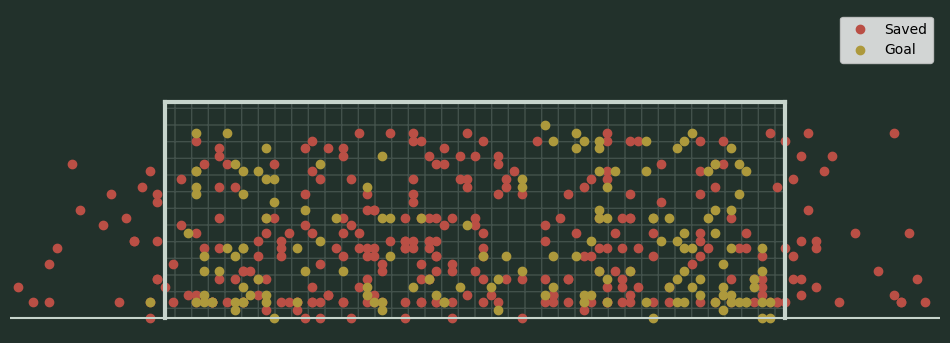
Every shot on target, based on end location of ball, and its result (Some are out of frame of goal because the ball was saved outside of the goals coordinates)


In order to build my xG model, I extracted data from every shot on target, and decided which features would be used for model building. The features that I settled upon include 'endz'(height of ball), 'shotangle'(calculated based on start and end location of ball), 'angle'(calculated based on start location of ball), 'distance'(calculated based on start location of ball), 'header'(binary), 'deflected'(binary), 'one_on_one'(binary), and 'technique_name'. My y variable was a binary variable ‘saved’, which would read 1 if a ball was saved and 0 for a goal.
After running a logistic regression on my data, my model presented these metrics: R² = 0.21829005468631357, MSE = 0.170244194204575, LogLoss = 0.5135122836438719. For reference, StatsBomb’s xG model produces an R² of approximately 0.24. However, it might be evident that this model has some serious oversights. Up to this point, the model only considers aspects about the shot itself. However, location and position of the goalkeeper would be equally as important when evaluating the probability of making a save. In order to understand this point better, I present to you every shot on target from the World Cup Finals, between Argentina and France, as well as my model’s xSave for each shot.

I immediately noticed that Emiliano Martínez’s game saving save, in the 122th minute was given an xSave of 0.828302. However, anyone who watches that save knows it is much lower than that, but when you consider that the model is only seeing that Kolo Muani was at the top of the box and hit a low shot to the bottom right side of the goal, it is clear to see how the model would consider this an easy save. For this reason, I knew I had to include goalkeeper metrics. After inspecting the data even, more I noticed that every shot on target has a following event logged from the goalkeepers perspective, which marks the outcome of the event as ‘Goal Conceded’ or ‘Shot Saved’. You can see this in the table below which displays the corresponding 12 shots on target from the goalkeepers perspective.

I was able to combine these two subsets of the data, by matching match ids as well as matching minute and second of the plays. Here is a look at what that dataset looks like

The dataframe above is exactly what was used to fit the new model. Angle, shot angle, and distance were again calculated using x_shot, y_shot, end_x, and end_y; while body_part_name and technique_name were converted to dummy variables. ‘x_goalie’, ‘y_goalie’, and ‘goalkeeper_position_name’ were the only fields added, as I felt they gave an inclusive understanding of the goalkeeper’s position and location. My new logistic model presented these metrics: R² = 0.24049479627728199, MSE = 0.16595005802934915, LogLoss = 0.5032282536584001. As you can see, the model improved in all three of these metrics.
I wanted to look at which goalkeepers overperformed and underperformed their expectations, so I grouped every shot on target by the goalkeeper that was in goal. After calculating the difference between xSave for the tournament and saves made, I sorted for top 10 by descending(left) and ascending(right). Here’s what I found:

Croatia’s Dominik Livakovic led goalkeepers in saves over expected by a decent margin, followed by Saudi Arabia’s Mohammed Khalil Al Owais. On the opposite end, Iran’s Seyed Hossein Hosseini, followed by Mexico’s Francisco Guillermo "Memo" Ochoa Magaña were bottom two in this statistic. To visualize their performance a bit more, I looked at their shot map to see where they were making saves and where they were allowing goals.

xSave of every goal conceded is listed above the point

Looking back at the example I provided earlier in this analysis, I wanted to compare the xSave of Emiliano Martínez’ last minute save in the world cup finals. This time we are given an xSave of 0.440325, a much more understandable value.

This is the first installment of Goalkeeper Analysis that I am working on. I intend to analyze the next main part of goalkeeping: distribution.